2uandtrilogy.com

Looking for tips to become an Excel pro?

No one can deny the importance of mastering Excel well in the office.

However, both beginners and experienced users do not necessarily know all the useful tips.

So here is 20 tips and tricks to turn you into a Microsoft Excel pro:

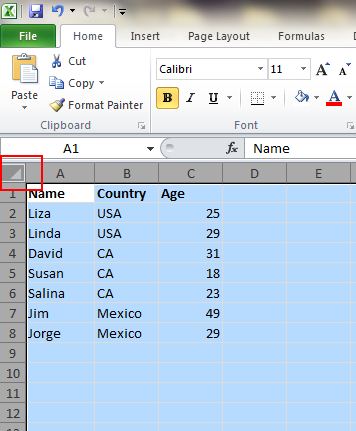
1. One click to select all

You may know how to select all cells using the Control (Ctrl) + A shortcut on your keyboard.

But not many users know that with just one click of the corner button, as shown below, all data is selected instantly.

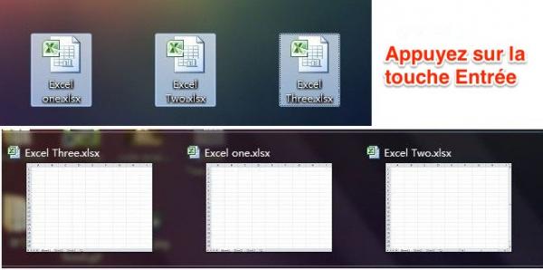
2. Open multiple files at the same time

When you need to use multiple files at the same time, instead of opening them one by one, there is a trick to open them all with 1 click.

Select the files you want to open and press the Enter key. All files will open simultaneously.

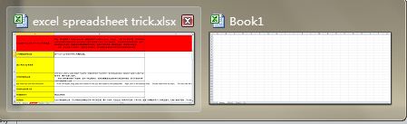
3. Switch between multiple Excel files

When you have multiple spreadsheets open, it's not very convenient to switch between them.

And if you have the misfortune of using the wrong file, you can compromise your entire project.

Use the Ctrl + Tab shortcut to switch between files easily.

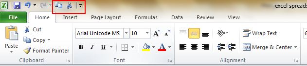
4. Add a new shortcut in the menu

By default there are 3 shortcuts in the top menu which are Save, Undo and Redo.

But if you want to use more shortcuts, like Copy and Paste for example, you can add them this way:

File -> Options -> Toolbar -> Quick Access and add Cut and Paste from left to right column and save.

You will then see 2 shortcuts added in the top menu.

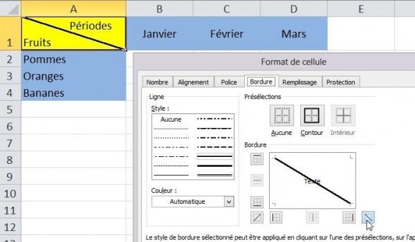
5. Add a diagonal line to a cell

When you create, for example, a list of customer addresses, you may need to make a diagonal dividing line in the 1st cell.

This is useful for differentiating between column and row information. But how do you do that?

Right click on the cell, then click on Format Cells, Borders, and finally on the button at the bottom right (downward diagonal) and validate.

6. Add multiple columns or rows at the same time

Surely you know how to add a new row or a new column.

But this method wastes a lot of time. Because you have to repeat the operation as many times as you have columns or rows to add.

The best solution is to select multiple columns or multiple rows, then right click on the selection and choose "Insert" from the drop-down menu.

The new rows will then be inserted above the row or to the left of the column you selected first.

7. Quickly move data from multiple cells

If you want to move a column of data in a worksheet, the fastest way is to pick the column and then put your pointer over the edge of the column.

And when it turns into a cross arrows icon, click on it and let press to freely move the column where you want.

What if you also need to copy the data? Just press the Control (Ctrl) key before moving the column. The new column will copy all the selected data.

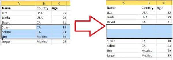
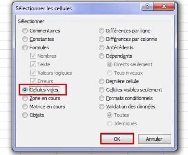
8. Quickly delete empty cells

When filling in information for work, sometimes there is missing data. As a result, some cells remain empty.

If you need to remove those empty cells to keep your calculations correct, especially when you are averaging, the fastest way is to filter out all the empty cells and remove them with 1 click.

Choose the column you want to filter, then click Data and Filter. Click Deselect and choose the last option named Empty Cells.

All empty cells are thus selected. You just have to delete them to make them disappear.

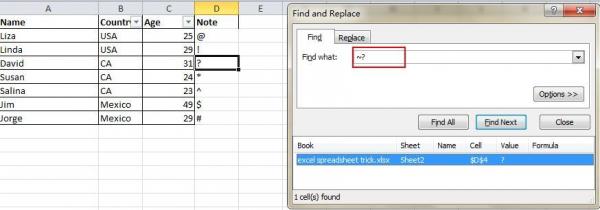
9. How to do a rough search

You might know how to turn on Quick Find using the Ctrl + F shortcut.

But did you know that it is possible to do a rough search using the symbols? (question mark) and * (asterisk)?

These symbols are for use when you are not sure what results you are looking for. The question mark is to be used to replace a single character and the asterisk for one or more characters.

And if you are wondering how to look for a question mark or an asterisk, just add the Wave symbol ~ in front of it like below.

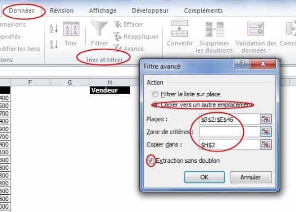
10. How to extract unique values ​​from a column

Have you ever had an array where you wanted to extract the unique values ​​from a column?

You are probably familiar with Excel's Filter function, but not many people use the Advanced Filter.

However, it is useful for extracting unique values ​​from a column. Click on the relevant column then go to Data -> Advanced. A pop-up will appear.

In this pop-up, click Copy to another location. Then choose where you want to copy the unique values ​​by filling in the Copy to field. To fill in this field, you can directly click on the area you have chosen. This avoids typing in precise values.

All you have to do is check the Extraction without duplicate box and click on OK. The unique values ​​will then be copied to the column you specified and can thus be compared with the data in the starting column.

For this reason, it is recommended that you copy the unique values ​​to a new location.

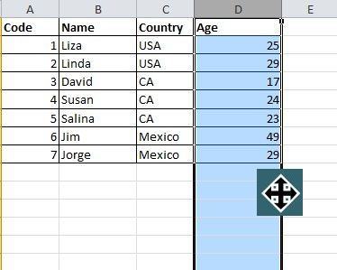
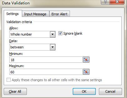
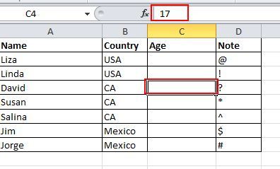
11. Restrict the data entered with the data validation function

To maintain data consistency, sometimes you need to restrict the values ​​that users can enter in a cell.

In the example below, the age of people must be a whole number. And everyone taking part in this survey must be between the ages of 18 and 60.

To ensure that participants outside this age group do not enter data, go to Data -> Data validation, and add the validation criteria.

Then click on the Input Message tab and enter a message like this "Please use a whole number to indicate your age. The age must be between 18 and 60 years old."

Users will thus receive this message when they hover their mouse over the affected cells and will have a warning message if the age entered is outside this age range.

12. Quick navigation with Ctrl + arrow button

When you click Ctrl + any arrow key on the keyboard, you can move to the 4 corners of the worksheet in the blink of an eye.

If you need to move to the last row of your data, try clicking Ctrl + down arrow.

13. Transform a row into a column

Need to display your data in columns while it is online?

No need to retype all your data. Here is how to do it.

Copy the area you want to turn into a column. Then place the cursor on the cell of the row where the data is to be placed.

Do Edit then Paste Special. Check the Transposed box and click OK. And there you have it, your data is now displayed in a column.

Note that this trick also works to transform a column into a row.

14. Hide data carefully

Almost all Excel users know how to hide data by right clicking and choosing Hide.

But the concern is that it can be easily seen if you have little data on the spreadsheet.

The best and easiest way to hide data neatly is to use a special cell format.

To do this, choose the area to be masked then right click to choose Format Cells.

Choose Custom and place the cursor in Type. Type the code ";;;" without quotes. Press OK. The contents of the cell are now invisible.

This data will only be visible in the preview area next to the Function button.

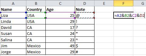
15. Combine the contents of several cells into 1 single

No need to use complicated formulas to combine the contents of multiple cells. As long as you know how to use the & symbol, you don't have to worry.

Below there are 4 columns with different text in each. But how do you combine them into 1?

Select a cell where you want to display the result. Then use the formula with the & as shown below on the screenshot.

Finally type Enter so that all the contents of A2, B2, C2 and D2 are combined into 1 single cell, which will give LizaUSA25 @.

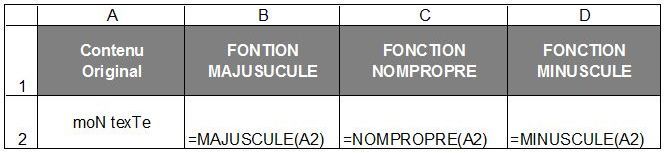
16. Change lowercase to uppercase letters

Want to change from lowercase to uppercase? Here is a simple formula to do it.

In the function field, just type CAPITAL as shown in the screenshot below.

And to change uppercase letters to lowercase, type SMALL. Finally to put a capital letter only on the 1st letter, type NOMPROPRE.

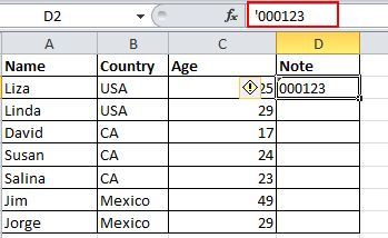
17. How to enter a value starting with 0

When a value begins with the number zero, Excel removes the zero automatically.

This problem can be easily resolved by adding an apostrophe before the first zero as shown below.

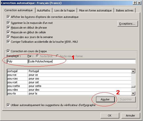
18. Speed ​​up entering complicated terms with autocorrect

If you need to type complicated text multiple times to type, the best way to do it is to use the AutoCorrect feature.

This function will automatically replace your text with the correct text.

Take, for example, École Polytechnique, which can be replaced by a simpler word to type such as Poly. Once the function is activated, each time you type Poly, it is corrected in École Polytechnique.

Convenient, isn't it? To activate this function, go to File -> Options -> Verification -> Automatic correction. Then fill in the text to replace with the correct text as shown below:

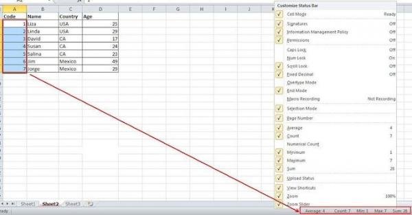
19. One click to get automatic calculations

Most people know that interesting information like Average and Sum can easily be obtained by glancing at the status bar at the bottom right.

But did you know that you can right click on this bar to get lots of other automatic calculations?

Give it a try and you will see that you have a choice.

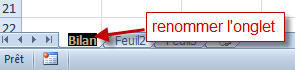
20. Rename a worksheet using double click

It has several ways to rename worksheets. Most people right click on it and then choose Rename.

But that wastes a lot of time. The best way to do this is to double click on the tab you want to rename and rename it here directly.

There you go, I hope you feel a little more comfortable with Excel now :-)

Note that these examples are based on Microsoft Excel 2010 but should also work well on Excel 2007, 2013 or 2016.

Where to buy Excel for cheap?

Looking to buy Microsoft Excel on the cheap?

So I recommend the Office 365 suite which includes Excel software. You can find it here for less than 65 €.

Also note that there are 100% free alternatives. Discover our article on the subject here.

Do you like this trick ? Share it with your friends on Facebook.

Also to discover:

The 5 Best FREE Software to Replace Microsoft Office Pack.

How To Make Keyboard Symbols: The Secret Finally Unveiled.